Mastering the Calculation: The Step-by-Step Guide to Finding Standard Deviation of Any Data Set
Mastering the Calculation: The Step-by-Step Guide to Finding Standard Deviation of Any Data Set
Standard deviation is the mathematical heartbeat of data analysis, quantifying how spread out individual values are from the mean. Whether assessing test scores, financial returns, or scientific measurements, this essential metric transforms raw data into actionable insight. Understanding how to compute standard deviation empowers analysts, researchers, and data enthusiasts to interpret variability with precision and confidence.
This article walks through every stage of the process—from gathering your dataset to applying the formula—so you can confidently measure dispersion like a seasoned statistician.
At its core, standard deviation reveals the degree of variation in a dataset. A low value indicates data points cluster closely around the mean, signaling consistency.
High values expose rich diversity or volatility, critical in risk assessment and decision-making. “Standard deviation transforms abstract numbers into tangible understanding,” explains statistician Dr. Elena Torres, author of The Analytics Edge.
“It answers the fundamental question: how predictable is the outcome?”
1. Gather Your Data: The Foundation of Accurate Calculation
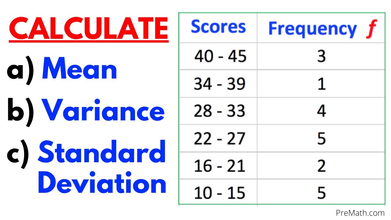
To find standard deviation, begin with a complete, well-organized dataset. This dataset can be a list of individual values—such as monthly sales figures, student exam scores, or sensor readings—or summarized from larger samples.For practical example, consider a small set representing weekly internet speeds (in Mbps): [25, 27, 26, 24, 29, 25, 28]. This sample contains seven observations and forms the basis for learning the full process.
Without reliable data, even the most sophisticated formulas yield misleading results. Always verify sources and clean entries of errors before proceeding.
2.
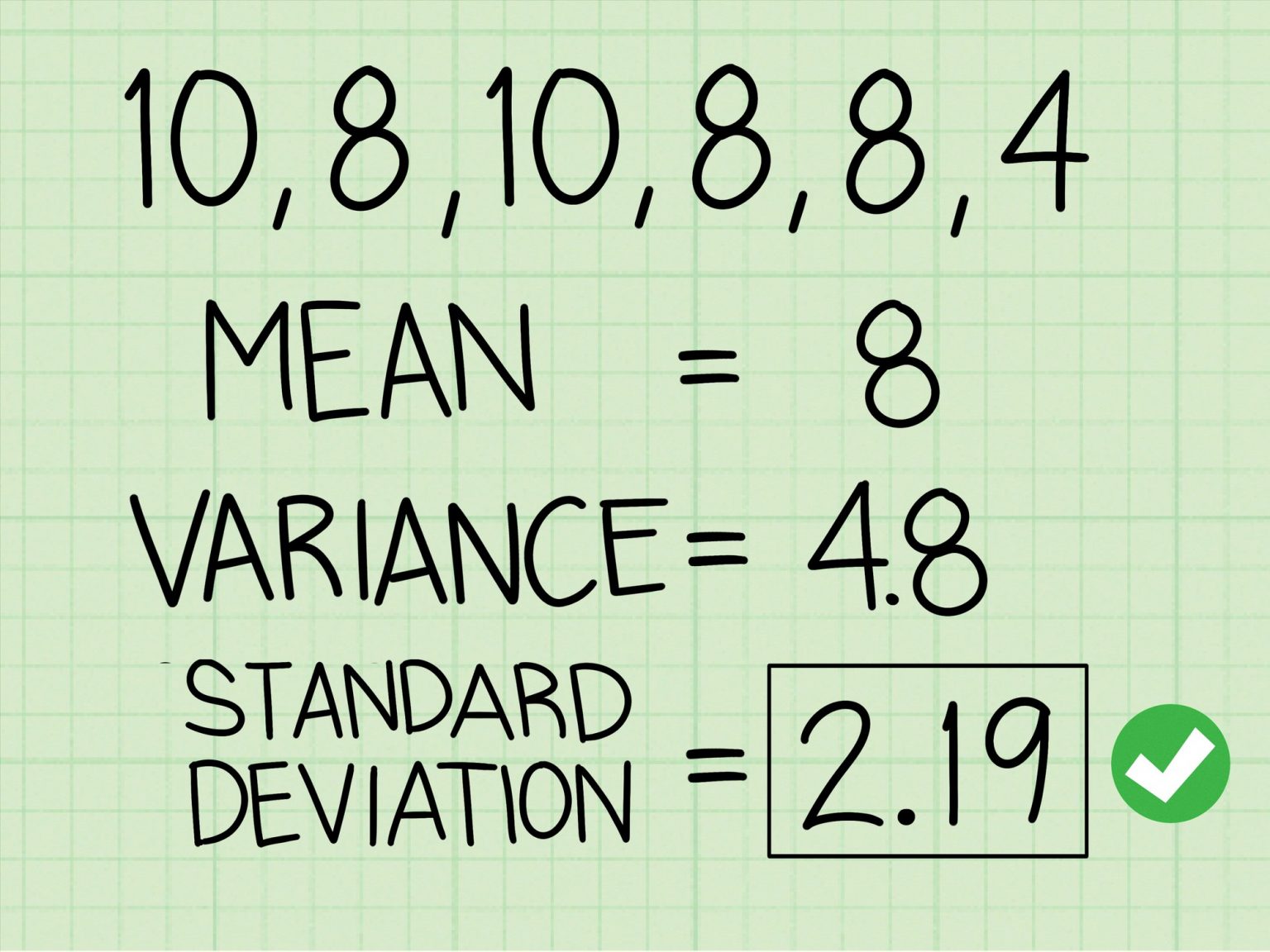
Calculate the Mean: The Center of Your Data Range The first mathematical step is computing the mean—the arithmetic average of all values. Add every data point, then divide by the total number of entries. For the speed dataset:
Sum = 25 + 27 + 26 + 24 + 29 + 25 + 28 = 184 Mean (μ) = 184 ÷ 7 ≈ 26.29 Mbps The mean serves as the reference point from which all other data points are measured relative to the center of distribution.Any deviation from this value—the critical input for standard deviation—must be calculated with precision.
3. Determine Deviations: Measuring How Far Each Value Falls from the Mean
With the mean established, evaluate how much each data point differs from the average.For each value, subtract the mean from the observation: Deviation = Observed Value – Mean Using the speed data: [25 – 26.29 ≈ –1.29, 27 – 26.29 ≈ 0.71, 26 – 26.29 ≈ –0.29, 24 – 26.29 ≈ –2.29, 29 – 26.29 ≈ 2.71, 25 – 26.29 ≈ –1.29, 28 – 26.29 ≈ 1.71] These deviations highlight the direction and magnitude of imbalance from the central tendency. Negative values indicate below-average performance or lower readings, while positive values signal above-average deviations.
Each deviation quantifies the distance between an observation and the teampoint—the mean.
But raw deviations alone don’t reveal spread; they must be standardized to account for scale.
4. Square the Deviations: Eliminating Negative Distances
To eliminate directional bias and emphasize magnitude, square each deviation. Squaring ensures all values are positive and amplifies larger discrepancies, which is crucial for accurate dispersion measurement: Squared Deviation = (Observed – Mean)² Applying to the deviations: [1.66, 0.50, 0.08, 5.24, 7.34, 1.66, 2.92] This transformation prevents positive and negative deviations from canceling each other out, focusing attention not just on how far data is from the mean, but how far it truly diverges.“Squaring converts raw spread into a meaningful scale,” clarifies Tom Reynolds, data scientist at Insight Analytics. “It sets the stage for the final step: averaging these squared differences.”
The Variance: Aggregating Squared Dispersions
The sum of squared deviations represents total variability across the dataset—but to express dispersion in consistent terms, this quantity is averaged. Divide the sum (32.21 in this case) by the number of observations (7), yielding the sample variance, denoted as s²: s² = Σ(x – μ)² / (n – 1) = 32.21 ÷ 6 ≈ 5.37 Using Bessel’s correction (n–1 instead of n), analysts correct bias in sample estimates—though for large datasets, the difference becomes negligible.The resulting variance (5.37 Mbps²) quantifies average squared distance but remains in squared units, limiting interpretability.
5. Take the Square Root: Restoring Original Units and Revealing Dispersion
Because variance uses squared units, standard deviation must be expressed in the same units as the original data to remain intuitive.Take the non-negative square root of the variance: Standard Deviation (s) = √Variance = √5.37 ≈ 2.32 Mbps This final figure represents how much, on average, data points deviate from the mean. In this example, speeds vary roughly 2.32 Mbps from the monthly average. “Standard deviation returns the answer to our core question: what is the typical spread?” notes Dr.
Torres. “It’s the natural language of uncertainty in data.”
To visualize, place this dispersal measure alongside the mean on a number line. The vertical distance from 26.29 to ±2.32 defines consistent observations; values beyond ±2.32—such as the 24 Mbps and 29 Mbps extremes—fall into the “outlier” zone, signaling higher volatility poles.
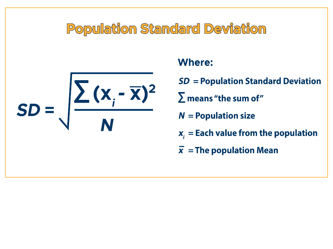
Different Datasets: Population vs. Sample – Why It Matters
The formula for standard deviation shifts slightly depending on whether the dataset represents a full population or a