How to Find the Y-Intercept: Master the Graph & Equation Like a Pro

Understanding the Y-intercept is fundamental to interpreting linear relationships in mathematics and data analysis. It represents the point where a line crosses the vertical axis—where the x-value equals zero—offering critical insight into a function’s behavior at rest. Whether solving equations, analyzing real-world trends, or building predictive models, knowing how to identify and extract this pivotal value ensures clarity and precision in technical work.

Mastering the process involves both algebraic manipulation and graphical analysis, forming the backbone of effective data interpretation.

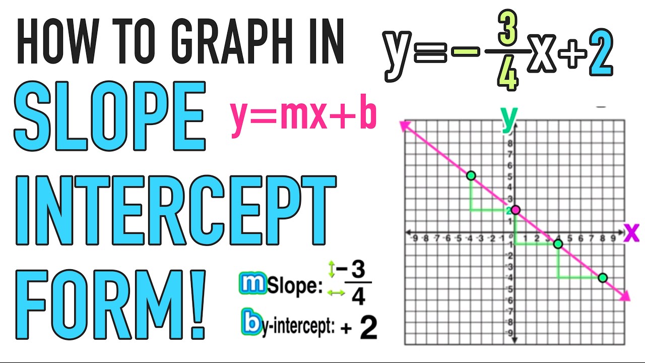
At its mathematical core, the Y-intercept of a line is defined as the value of y when x = 0. Expressed algebraically, for a linear equation in slope-intercept form y = mx + b, the Y-intercept is simply the constant term b.

This simplicity belies the importance of verifying this value in different contexts—whether deriving it directly from an equation, extracting it from a graph, or calculating it via regression in statistical models. “The Y-intercept anchors a line in context,” notes Dr. Elena Marquez, applied mathematics professor at Georgetown University.

“It tells us what the system measures when input is zero—without it, interpretation remains incomplete.”

Step-by-Step Guide to Determining the Y-Intercept
Across contexts, the method for finding the Y-intercept follows a logical sequence, though execution varies based on available data. The primary approaches include direct extraction from algebraic equations, graphical interpretation from coordinate graphs, and leveraging linear regression models for dataset analysis. Each technique provides a reliable path to the same essential measurement.

1.

From Algebraic Equation
For equations explicitly written in y = mx + b, isolating b delivers the Y-intercept instantly. This relies on the slope-intercept form, where b is the lone constant. For example, the line y = -3x + 5 has a Y-intercept at y = 5—the point (0, 5).

Not all equations use this form, but rearranging into standard linear format remains the first analytical step.

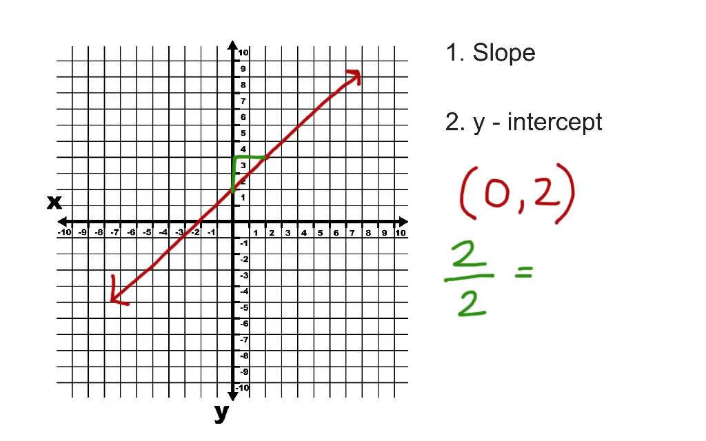
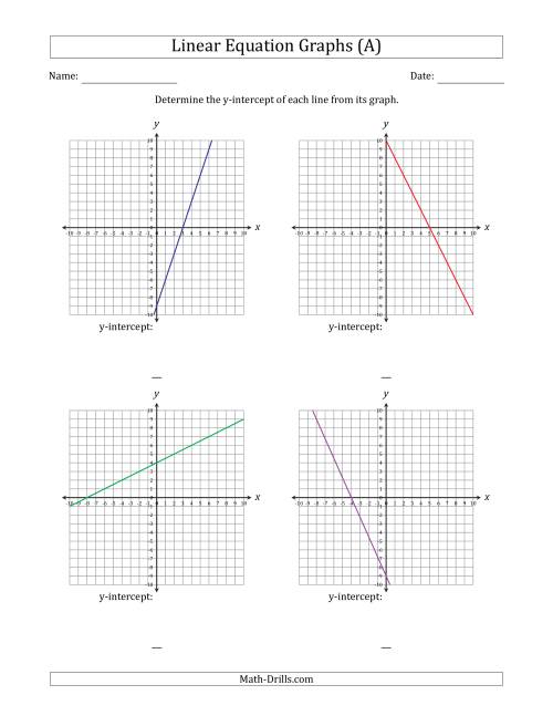
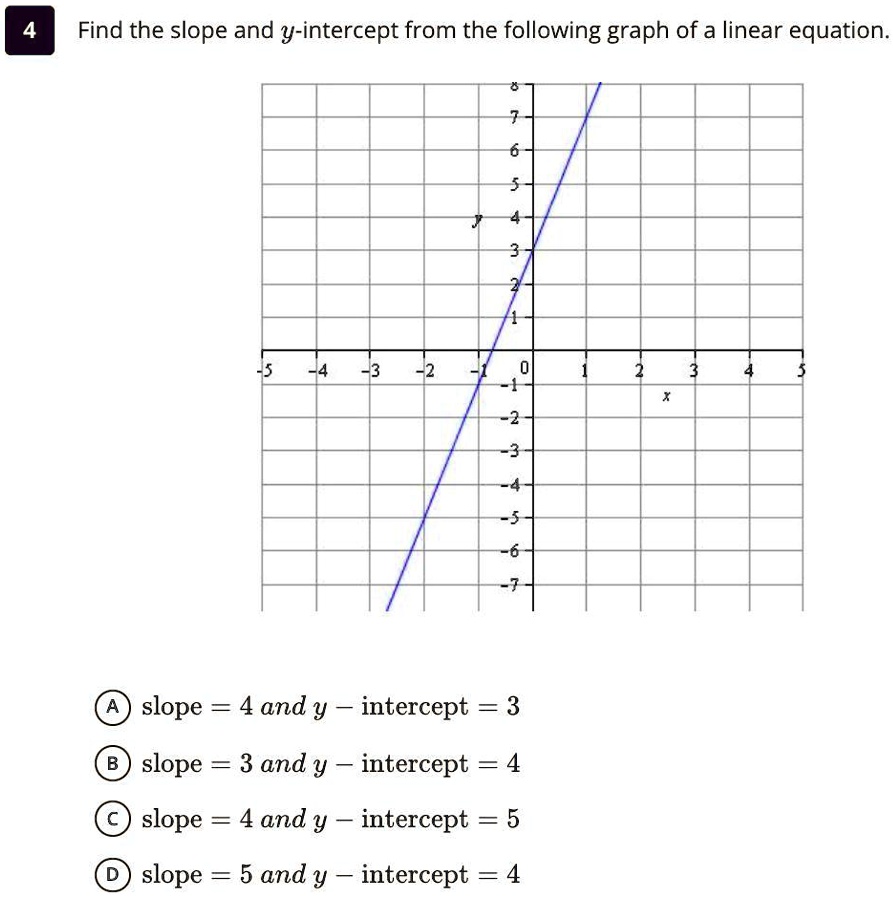
2. Using a Graph of the Line
On a coordinate plane, locate where the line crosses the y-axis—between the origin (0,0) and upward or downward along the vertical axis. This visual method confirms the intercept even when not given algebraically.

Suppose a plot shows a line passing through (0, -4) and (2, -2); the Y-intercept, confirmed geometrically, is clearly at (0, -4). Accuracy improves with careful graphing tools or digital platforms that allow precise point plotting.

3. Through Linear Regression Analysis
In data science and statistics, datasets often require derived intercepts via regression.

Using statistical software or calculators, input x and y values to compute the best-fit line, with the Y-intercept emerging as a key parameter. For instance, a dataset of monthly temperature readings plotted over a year might yield a regression model with equation T = -0.8m + 22.5, where m = -0.8 is the slope and b = 22.5 the Y-intercept—signaling a baseline temperature when m = 0 (month zero, typically January). This approach extends to non-perfect fits, offering robust extraction even with noisy data.

4.

From Two Points Using Slope Calculation
When given only two points on a line—say, (2, 3) and (4, 7)—the slope m = (7-3)/(4-2) = 2 is computed. With m known, substitute either point into y = mx + b to solve for b. Using (2,3): 3 = 2(2) + b → b = 3 - 4 = -1.

Thus, the Y-intercept is (0, -1), reinforcing that slope and intercept are inseparable in linear systems.

Best practices emphasize cross-verification: regardless of method, confirming the result through multiple approaches prevents errors, especially critical in applications like financial forecasting, engineering design, or environmental modeling. “Always triangulate the Y-intercept,” advises Ravi Desai, data analyst at the National Institute for Statistical Research. “Confirm it algebraically, visually, and analytically to build confidence in your model’s foundation.”

Common pitfalls include confusing Y-intercept with x-intercept (“the X value when Y is zero”), misreading graphs due to scale distortion, or relying solely on estimation without verification.

Being exact here avoids cumulative errors that cascade through calculations, especially in iterative processes like machine learning model tuning or policy impact analysis.

In advanced contexts, the Y-intercept also serves as a convergence point in systems modeling—where multiple variables stabilize at baseline conditions. It plays a role in predictive analytics, economic equilibria, and even signal processing, where zero input reveals intrinsic system behavior. Recognizing and accurately determining this simple yet profound value transforms raw data into actionable knowledge.

The Y-intercept, though mathematically straightforward, is indispensable across disciplines. From classroom equations to real-world datasets, mastering its identification ensures analytical precision and deepens understanding of linear relationships. Whether calculating directly, graphing, or computing via regression, the core principle remains: locate y when x rests firmly at zero.

In doing so, one unlocks a critical node in data and equations—foundational, reliable, and endlessly applicable.