Decoding Swift Swaps: The precise art of Python-driven interest rate swap pricing

In the high-stakes world of financial markets, precision governs every transaction—and nowhere is this more critical than in interest rate swap pricing. These complex instruments hinge on delicate calculations that determine long-term cash flows between fixed and floating rate counterparties, making accurate valuation not just a technical necessity, but a financial imperative. Enter Python: a powerful, accessible, and increasingly indispensable tool that transforms theoretical pricing models into real-world applications.

This guide reveals how Python is reshaping the economics of swap valuation—from raw data input to final market-transformed pricing—offering practitioners clear, actionable insights grounded in both theory and implementation.

Understanding The Mechanics: How Interest Rate Swaps Work

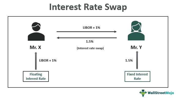
At its core, an interest rate swap is a derivative contract where counterparties exchange interest payments—typically one paying a fixed rate and the other a floating rate, often tied to benchmarks like LIBOR or SOFR—over a defined term. These swaps enable firms to manage exposure, optimize financing costs, and gain strategic positioning in volatile rate environments.

Physically, a swap consists of two legs: - The **fixed-rate leg**, where cash flows remain unchanged over time - The **floating-rate leg**, where payments fluctuate with prevailing market rates, most commonly scaled to a risk-free rate plus a spread The net payment differential between legs forms the swap’s economic value at any point in time, forming the basis for quantitative evaluation.

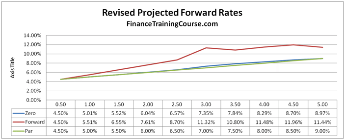
Pricing a swap isn’t merely about matching cash flows—it demands modeling the term structure of interest rates, projecting future rates with realism, and discounting expected payments to present value using appropriate yield curves. This multidimensional process calls for automation, speed, and accuracy—qualities that Python delivers in abundance.

Why Python Reigns Supreme in Swap Pricing

While spreadsheets and legacy systems once dominated, Python has emerged as the preferred language for modern swap valuation.

Its strengths include: - **Flexibility**: Support for custom models, sensitivity analysis, and scenario testing - **Rich libraries**: NumPy, SciPy, Pandas, and QuantLib provide robust tools for numerical computation and fixture modeling - **Open-source transparency**: Full visibility into formula logic enables auditability and validation - **Integration capability**: Seamlessly connects with real-time data feeds, risk engines, and trading platforms “Python democratizes quantitative finance,” says Dr. Elena Torres, Quantitative Analyst at Aspect Financial. “What once required custom-built software or laborious manual reformulation is now achievable with well-documented, reproducible code—inside hours, not weeks.”

From static prepricing to dynamic Monte Carlo simulations, Python handles complexity with elegance, turning abstract financial theory into tangible, executable code.

Core Components of a Swap Pricing Engine in Python

Building a reliable Python-based swap pricing system requires attention to four essential building blocks:

1.

Discounting Mechanics

Market outcomes depend on discount factors derived from a chosen yield curve—most often the projected forward curve for floating legs. Using bootstrapped zero-curve estimates, Python computes present values of future cash flows with precision. Libraries like `wendliche` and `pyrs` simplify this process, supporting both physical and risk-adjusted discounting.
Software experts emphasize: “Accurate discounting is the backbone of swap pricing,” notes Rajiv Mehta, Fixed Income Developer at FinTech Solutions.

“Python’s ability to iterate on curve constructions and stress-test discount factors gives our pricing models a resilience few alternatives match.”

2. Cash Flow Generation

Each leg’s payments must be projected forward—tacking accruals, compounding interest, and applying day-count conventions with millimeter precision. Python’s datetime and calendar utilities enable sophisticated timing logic, while symbolic math libraries (SymPy) allow symbolic manipulation of future value formulas.

Example workflow: - Init fixed fixed-resistance CDY curves - Simulate floating rate benchmarks using forward rate agreements - Compute each period’s floating cash flow based on accruals and payments frequency

3. Modeling Market Variability

Swap valuations are not static. VaR analysis, sensitivity to rate shocks, and scenario tests demand robust statistical modeling.

Python’s ecosystem accelerates this with Monte Carlo frameworks and stochastic volatility models. Realistic rate path simulations incorporate correlation structures, turbulence, and regime shifts—critical for risk assessment and regulatory reporting. One common Python construct for sensitivity analysis: ```python import numpy as np from scipy.stats import norm def swap_sensitivities(rate_sim, fixed_rate): delta_vals = np.diff(rate_sim) vega = np.cov(delta_vals, np.ones_like(delta_vals))[0,1] * np.std(delta_vals) / np.mean(delta_vals) gamma = np.var(rate_sim) / np.mean(delta_vals)**2 return {'vega': vega, 'gamma': gamma} ```

4.

Calibration and Market Consistency

To align models with real-world dynamics, prices must calibrate against market quotes—swaptions, caps/floors, freight curves. Python automates this calibration via optimization routines: minimizing residual errors between model and market values using low-level solvers from `scipy.optimize`. A typical calibration loop minimizes the objective function: \[ \min_\theta \sum_i (P_{\text{model}}(t,\theta) - P_{\text{market}}(t,\theta))^2 \] This iterative process ensures that simulated futures remain anchored in current market realities.

Implementing a Baseline Swap Pricing Model

Consider a simple plain vanilla swap: five-year tenor, fixed at 3.5%, floating tied to SOFR. Using Python, a minimal but robust pricing engine proceeds as follows:

Step 1: Build the discount curve

Using daily cash flow data, construct a zero-zero yield curve with bootstrapping.

Step 2: Project floating payments

For SOFR-linked floating, project weekly or quarterly rates with LIBOR-Euribor spread dynamics, and apply accrued interest for partial periods.

Step 3: Calculate expected floating PV

Discount projected floating cash flows to present value using the curve.

Step 4: Compute net payment

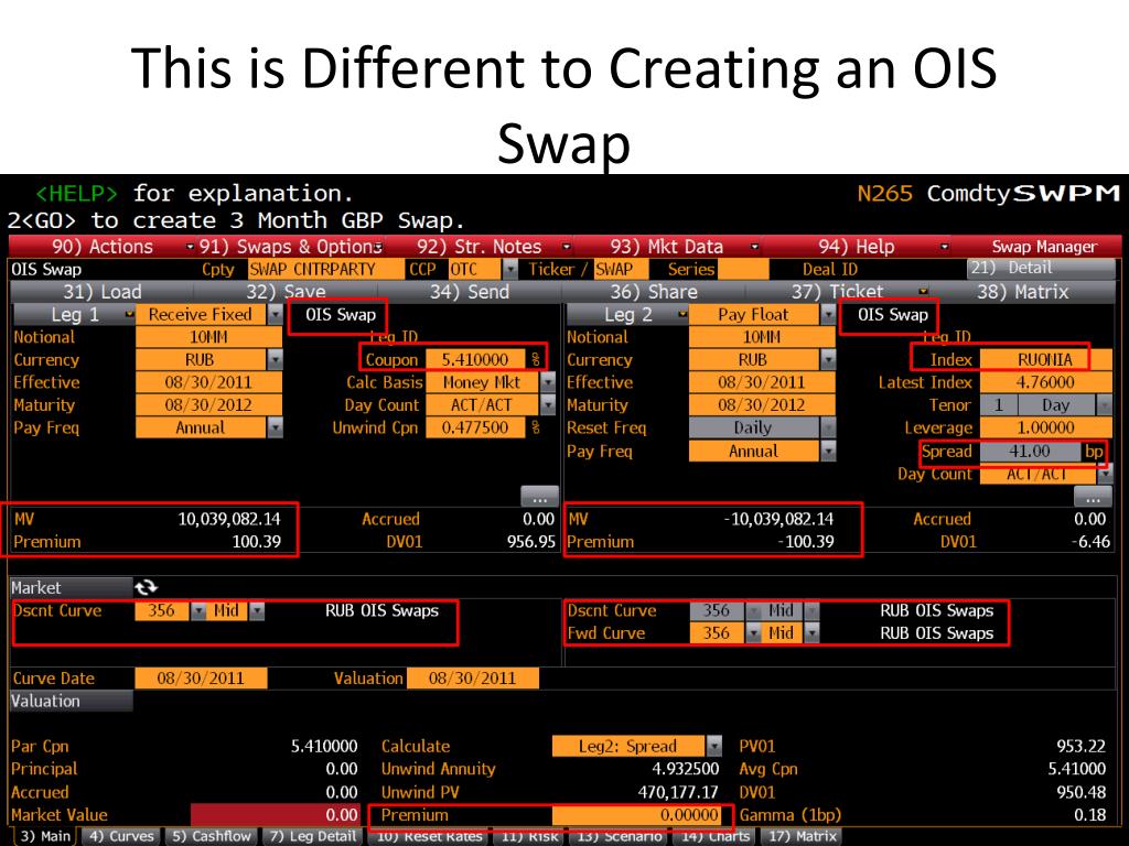
Subtract fixed leg value (sum of fixed payments) from floating PV. This process repeats under different curve scenarios—Hagrangian bootstraps, LIBOR reformulation, OIS transitions—enabling full flexibility for risk analysis.

For practitioners executing these steps, Python’s readability accelerates collaboration across risk, quant, and trading teams, reducing bugs and accelerating time-to-insight.

Advanced Techniques: Stochastic Modeling and Monte Carlo Simulations

For exotic swaps or path-dependent valuations, deterministic discounting falls short. Here, stochastic interest rate models—such as Hull-White, Black-Derman-Toy, or LIBOR Market Models—integrate seamlessly into Python. These models simulate thousands of rate paths, calculate forward rates under risk-neutral measures, and aggregate net payoffs across scenarios.

Monte Carlo’s power lies in variance reduction techniques—antithetic variates, control variates, importance sampling—each implementable in Python to boost efficiency. Importantly, the language’s Jupyter notebook ecosystem supports interactive exploration, allowing analysts to visualize interest rate manifolds,ヒ热销热销 heat maps, and sensitivity heatmaps in real time. “Monte Carlo in Python isn’t just about speed—it’s about clarity and adaptability,” remarks Dr.

Leonor Cruz, Senior Quant at QuantMetrics. “With custom-built modules, we simulate complex dynamics while maintaining audit trails—essential for both trading decisions and compliance.”

The Role of Automation and Integration

Python-based swap pricing engines thrive when integrated into automated pipelines. Feed FX or central bank rate feeds live, trigger daily re-pricing, update P&L statements, and push valuation outputs directly to P&L systems.

Tools like Apache Airflow orchestrate execution schedules, error handling, and logging—turning static reports into dynamic dashboards. Real-time integration also enables live risk calculation—monitoring DV01, exposure shifts, and collateral requirements across portfolios. Importantly, Python’s interoperability with C++, Java, and financial APIs ensures minimal friction when embedding pricing models into existing infrastructure.

Best Practices and Common Pitfalls

Adopting Python in swap pricing demands discipline. Key best practices include: - Maintain version control with Git to track model evolution - Unit test critical components—especially discount factor and cash flow generators - Benchmark Python results against trusted sources or legacy systems - Document all assumptions, particularly curve selection and day count conventions Avoid common oversights: - Ignoring non-paridade spreads or slippage in floating leg modeling - Neglecting floating rate accrual timing, leading to cash flow mismatches - Overlooking liquidity premiums or credit adjustments in real-world pricing “Consistency is king,” stresses Rajiv Mehta. “Elements like day counting, compounding, and payment alignment must be rigidly enforced—Python helps codify these rules, reducing error margins to near-zero.”

Conclusion: Python as the Engine of Modern Swap Pricing

From fixed versus floating valuation amid volatile rate environments, Python has evolved from tool of choice to essential infrastructure in interest rate swap pricing.

Its combination of computational precision, model flexibility, and seamless integration enables financial professionals to calculate, analyze, and act with unprecedented speed and reliability. As markets grow more complex, the edge lies not just in theory—but in code, automation, and continuous model refinement—with Python leading the charge. Practitioners who master its nuances transform pricing from a compliance chore into a strategic asset, driving smarter risk management and more resilient financial outcomes.